Constructing BPEL processes using
GRASS webservices
To be able to create BPEL processes using GRASS webservices, it is good to have a user level knowledge of GRASS software and introductory knowledge of BPEL. Almost all of the GRASS webservices emulate a GRASS command. To use any GRASS webservice, one just needs to know the corresponding GRASS command. All the GRASS commands are listed in the following webpage under the heading ˇ°Manual Sectionsˇ±:
http://grass.itc.it/grass61/manuals/html61_user/index.html
Later on, I will explain how each command maps to a web service. First let us look at the basics of GRASS architecture, which are sufficient to get started. One does not need to know whole lot about GRASS, just the following is enough to begin:
ˇ°GRASS data are stored in a directory referred to as DATABASE (also called ``GISDBASE''). Within this DATABASE, the projects are organized by project areas stored in subdirectories called LOCATIONs. A LOCATION is defined by its coordinate system, map projection and geographical boundaries. The subdirectories and files defining a LOCATION are created automatically when GRASS is started the first time with a new LOCATION. Each LOCATION can have several MAPSETs. One motivation to maintain different mapsets is to store maps related to project issues or subregions. Another motivation is to support simultaneous access of several users to the map layers stored within the same LOCATION, i.e. teams working on the same project. For teams a centralized GRASS DATABASE would be defined in a network file system (e.g. NFS). Besides access to his/her own MAPSET, each user can also read map layers in other users' MAPSETs, but s/he can modify or remove only the map layers in his/her own MAPSET. When creating a new LOCATION, GRASS automatically creates a special MAPSET called PERMANENT where the core data for the project can be stored. Data in the PERMANENT MAPSET can only be added, modified or removed by the owner of the PERMANENT MAPSET; however, they can be accessed, analyzed, and copied into their own MAPSET by the other users.ˇ± (GRASS manual)
GISDBASE, LOCATION and MAPSET are the variables which are passed to all GRASS webservice which emulates the corresponding GRASS command. Each and every raster coverage is stored in a MAPSET within a single LOCATION and a GISDBASE. These three variables, in a way, store the state information. Webservices are supposed to be stateless. But in this case, that property is by passed using the arguments which store the state information. We will see later on, that process workflows (which are composed of several webservices and are webservices themselves ) can be made completely stateless (This leads one to believe that GRASS services are better designed as stateful GRID services and workflows as stateless webservices). These higher level process workflows are equivalent to GRASS scripts which contain several GRASS commands that are executed together. So creating processes using the GRASS webservices is equivalent to creating a GRASS script. But unlike GRASS script, the processes can make use of other non-GRASS web services. Also, there is lot of scope for parallelization of various tasks. There are whole lots of other benefits.
We will look at a simple example to get an idea about how the GRASS webservices are structured and how they can be used to create higher level processes. We will create a simple process to calculate NDVI from two raster data files (NIR and Red Images). The inputs to the process are the two images- NIR and Red Image and the output is a single image containing NDVI values. Let us assume that the input images are in the GeoTiff format.
A person, who worked with GRASS, will probably follow the following steps to get the NDVI values:
1) Create a directory which represents a GRASS database.
2) Create a new LOCATION and MAPSET into which the images will be imported. There are two cases now:
a) You know the projection and datum and bounding box of the input images. And will use this information in creating location.
b) The more general case is you donˇŻt have any information about the projection or bounding box of the input images and you want to create a new LOCATION by reading the metadata present in the input images.
Let us consider the more general case. For this, you create a dummy location and mapset with any projection and datum. From within this location, use r.in.gdal command to import any one of the two images into a new location. (For those you, who donˇŻt know GRASS, r.in.gdal is a very special command, which can import large number of data formats into GRASS database. Also it has an optional argument (called location), which can be used to read the metadata from the input file and use it for the creation of a new location. Please see : http://grass.itc.it/grass61/manuals/html61_user/r.in.gdal.html for more information.).
3) Exit the GRASS and enter the new location. Import the second image using r.in.gdal once again without location option.
4) Using r.mapcalc to perform arithmetic on the raster maps to calculate ndvi values. (The command may look something like this:
r.mapcalc "ndvi=float(lsat.4 - lsat.3) /
(lsat.4 + lsat.3)". r.mapcalc is another very useful GRASS command. Please
see: http://grass.itc.it/grass61/manuals/html61_user/r.mapcalc.html
for more information)
5) Use one of the
raster export commands to export the resulting image into a file. Let us say
you want the image in png format. Use r.out.png to export the raster file
into png format. (Please see: http://grass.itc.it/grass61/manuals/html61_user/r.out.png.html
for more information about r.out.png.)
Now we will create a BPEL workflow which will do the same thing as above. For each step above, there is an analogous step in the BPEL workflow:
1) The directory which represents a GRASS database is automatically created when you create a new location using create_dummy_location service in the next step. So you donˇŻt have to do anything in this step. (Alternatively, you can use create_location service if you know the projection and bounding box of the input images.)
2) Use create_dummy_location service to create a dummy location. This service creates a new GRASS database and a dummy location within the database. The input to this service is the name of the dummy location you want to create (it could be any). The output to the service is the name of the GRASS database which is created by the service.
Call r_in_gdal service with one of the images as an input, to create a new location which has the projection and bounding box read from the input image. For the input image, the url of the image file is the input (and not the path of the input file).
This step is equivalent to calling these two calling these two functions:
String
gbase=create_dummy_location(ˇ°templocˇ±);
r_in_gdal(gbase,ˇ±templocˇ±,ˇ±PERMANENTˇ±,false,false,false,false,
ˇ°http://geobrain.laits.gmu.edu:8099/temp/TMImage/TMBand3.hdfˇ±,ˇ±NIRImageˇ±,null,null,null,ˇ±newlocˇ±);
Note the similarity of the GRASS webservice with the corresponding GRASS command:
GRASS command:
r.in.gdal [-oefk] input =string output=string
[band=integer ] [target=string] [title=string]
[location =string]
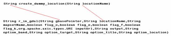
Corresponding GRASS webservice:
public String
r_in_gdal(String gbasePointer,String locationName,String mapsetName,boolean flag_o,boolean
flag_e,boolean flag_f,boolean flag_k,org.apache.axis.types.URI inputUrl,String
output,String option_band,String option_target,String option_title,String
option_location) throws java.rmi.RemoteException,edu.gmu.laits.ws.WebServiceExceptionsType;
All the arguments which represent flags in the command have ˇ°flag_ˇ± as their prefix, all the optional arguments have ˇ°option_ˇ± as their prefix and the mandatory arguments donˇŻt have any prefix. Whenever the input argument to the GRASS command is an operating system file, the corresponding argument in the webservice is a URL. Whenever the output from a GRASS command is an operating system file, the output from the corresponding webserivce is a URL which is created on the server. Sometime, the input(or output) may be directories rather than files (e.g. ARC/INFO coverages), in such cases, the webservice expects (or outputs) a zip file containing the raster coverage. Please see the following website for how to interpret arguments in a GRASS webserivce:
http://geobrain.laits.gmu.edu:8099/webservices/grass/Grass_Webservices.html
3) Use r_in_gdal service to import the other image into the GRASS database.
r_in_gdal(gbase,ˇ±newlocˇ±,ˇ±PERMANENTˇ±,false,false,false,false,
ˇ°http://geobrain.laits.gmu.edu:8099/temp/TMImage/TMBand4.hdfˇ±,ˇ±RedImageˇ±,null,null,null,null);
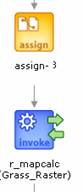
4) Use r_mapcalc service to create an NDVI image within the database. This step is equivalent to calling this function:
r_mapcalc(gbase,ˇ±newlocˇ±,ˇ±PERMANENTˇ±
,ˇ±NDVIˇ±,ˇ± float(RedImage- NIRImage) /
(RedImage + NIRImage)ˇ±);
5) Use r_out_png service to export the NDVI image which is created inside the database in the previous step. The output is a URL containing the png image of the NDVI values. This step is equivalent to calling the following function:
org.apache.axis.types.URI
outputUrl= r_out_png(gbase,ˇ±newlocˇ±,ˇ±PERMANENTˇ±,false,ˇ±NDVIˇ±)
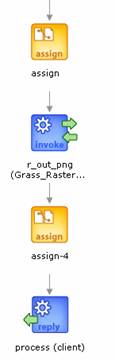
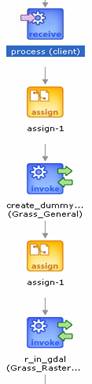
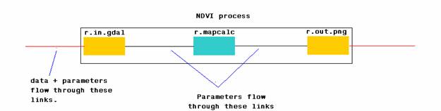
The output to this process is the image containing the NDVI values. The GRASS database, locations and mapsets created during the process are transient. As soon, as the process is complete, the database is invalid and can be deleted from the server. Database for each and every process is separate. In summary, the process workflow looks something like the figure shown below. The process itself is stateless, even though the services within have a state passed as arguments to the services.
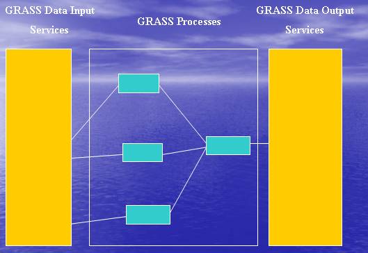
Most of the GRASS commands, like r.mapcalc (which is used for map algebra) have higher level meaning. They are best left as separate services. Most of the higher level functions like Supervised classification, Unsupervised classification, resampling, mosaicing, etc, can be achieved by using only a few GRASS commands (4 or 5 at the most). Therefore, I felt that it is better to convert each and every command into a webservice (Further this simplifies creation of webservice interfaces since software automation techniques can be used for creating interfaces). These web services can be combined in myriad different ways to create large number of complex processes. The figure below shows schematically, how a higher level process could be composed from GRASS web services.
Even though in the last example (NDVI example), I combined GRASS data input/output services with other GRASS services (r_mapcalc to be precise) to create a process workflows, it was only meant as an example. It is better to separate the input/output services from the actual workflow. That is process workflows are better created as a GRASS workflows, under the assumption that all the data is already in the GRASS database. This separation of GRASS workflows from input/output services ensures that the processes are independent of the input/output data formats. Depending on ones input/output data format requirements, one can quickly create a process by combining the right GRASS input and output service with the GRASS workflows. Or better yet, there is a scope for an intelligent webserivce which can input (or output) any data format. It is important to understand how the separation of core process workflow from the input/output websevices helps.
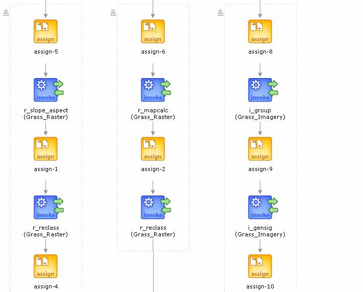
Next we will briefly look at how, some of the tasks can be parallelized. GRASS 6.0 allows multiple sessions. In GRASS, two different users can log into the same location but different mapsets simultaneously. Raster layers in different mapsets can be made accessible to each other. This property can be used to create massively parallel GRASS process workflows. I will explain this point with an example of a simple landslide model. Shown below in the figure of a landslide model:
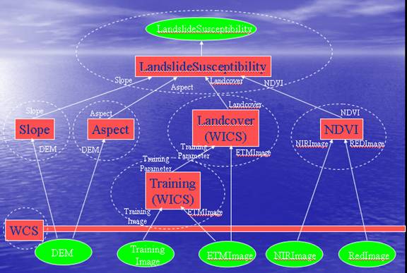
In this model, Landslide susceptibility is calculated by using four different parameters ¨Cslope, aspect, landcover and ndvi. Each of these parameters is calculated independently ( and hence each has a separate branch leading to landslide susceptibility). This means that workflow can be parallelized. Slope, aspect, landcover and ndvi can be created in a separate mapset, but the same location. Since GRASS allows parallelization in the same location but different mapsets, this property can be used to create processes which run in parallel. Also since rasters in any given mapset within a location can be made accessible to all the mapsets, landslide susceptibility can be calculated.
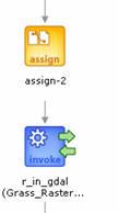
If we have access to computational cluster, operations on each mapset of the location
can made to be carried out by a different node of the cluster on which GRASS is installed. This leads to a scalable GRASS system. But GRASS processes should be written to make use of this scalability (or in other words, parallel branches in a workflow should run on different mapsets (and hence different nodes of the cluster)). The figure below shows a part of a landslide process workflow with each branch using a different mapset. Further work is need to see the feasibility of using the system for creating massively parallel workflows.