This Multiple-Protocol Geospatial Client (MPGC) User's Guide documents how to use MPGC, an interoperable system for accessing geospatial Web services, especially those from the Open Geospatial Consortium (OGC). These pages include descriptions of the user interface along with step-by-step instructions for completing specific tasks. Screenshots of tornado damage to illustrate the explanations through most of this guide's pages.

We assume that you are familiar with your operating system platform and with how to install a program.

1.2 What is MPGC

MPGC provides an interoperable way of accessing geospatial Web services, especially those from the Open Geospatial Consortium (OGC), for integrating and analyzing distributed heterogeneous Earth science data. MPGC utilizes the geospatial interoperability and Web service standards developed by the OGC, ISO, W3C, and GRID communities to enable service discovery, invocation, negotiation and selection. MPGC is in conformity with the OGC Catalog Service for Web (CSW) specification to play a “directory” role that permits the registry, discovery and access of geospatial information resources that are distributed on the Internet, such as services, data sets, data descriptions, and their associations. By implementing the latest protocols of the OGC Web Feature Service (WFS), Web Map Service (WMS) and Web Coverage Service (WCS), MPGC provides a single point of entry for access to OGC-compliant data services around the world, to request any subsets of multi-dimensional and multi-temporal geospatial data for a specific geographic region. It provides the capabilities to handle all the details of different protocols internally, so that users do not need to know the low-level details of the procedure for finding and accessing these data. MPGC also can access tool-like Web services, such as the Web Image Classification Service (WICS) and the Web Coordinate Transformation Service (WCTS), to produce value-added data products. Moreover, it also can 1) request any subset of multi-dimensional and multi-temporal geospatial data for a specific geographic region; 2) reformat the returning dataset in a data format specified by the user; 3) provide robust visualization and analytical tools for geospatial data; and 4) support multiple data formats: HDF, GeoTiff, GML, JPG, PNG, and GIF.

1.3 A Tornado Damage Example

Throughout this guide, we provide examples and screenshots from a tornado damage example:

· Data used:

1. AST_06S_003061820021605_DecorrelationStretchSWIR

2. TM classification

3. La Plata damaged area

· Bounding Box

UTM: 317600, 4246000, 341600, 4270000 (Note: the entire ASTER bounding box: 280835, 4213852, 36403, 4291236)

· Procedure:

1. Get ASTER data bands 5,7, and 9 (band 5 B/W shows a good tornado scene) from WCS

2. Make a color composite of the three bands

3. Get La Plata snapshots using WFS

4. Query snapshot feature and click http link to show photos

5. Get TM classification using WCS

1.4 System Requirements

The MPGC is distributed in No_VM_bundled which does not contain the Java Runtime Environment (JRE). To run MPGC, JDK1.4.x is required. MPGC does not compile on jdk1.3.x or earlier version. It may run on JDK 1.3.x but it is not tested on jdk1.3.x. Download Java 2 Platform at http://java.sun.com/j2se.

The MPGC uses the HDF Java Native Interfaces, which calls the HDF library. These native interfaces are included in the distribution. For more information (source and pre-built) on the HDF4/5 Java Native Interface, visit website at http://hdf.ncsa.uiuc.edu/hdf-java-html/JNI/.

MPGC 1.0 has been built and tested on the windows XP platforms. We will release a Solaris version in the future.

1.5 Installation

The source and pre-built binaries for MPGC can be downloaded from
http://geobrain.laits.gmu.edu/mpgc/. After downloading, double-click mpgc.exe. The installer will guide you to select the MPGC directory in which you want to install the MPGC). After the MPGC is installed, it can be launched from the desktop or Start -> Program Files -> MPGC.

Note: before you install the MPGC, you must have JDK1.4.1 or JDK1.4.2 installed on your machine. If you don't have a Java 2 VM, you must download and install one.

After downloading, double-click mpgc.exe

2. Getting Started

This chapter assumes that you have installed MPGC.

2.1. The Main Window

When you first open MPGC, the MPGC window appears with an empty tree and data panel. After you open a project or file, the structure of the project and related file is displayed in the Tree Panel. The content of a data is displayed in the Data panel.

The main window consists of five components: Menu bar, Tool bar, Project tree panel, Data Panel, and Info panel.

Figure 1. Main Window

2.1.1. Menu bar

The menu bar is at the top of the main window. You can select a menu command from the menu items or press a key combination from the keyboard to invoke the menu item's action without navigating the menu hierarchy. For example, to exit the MPGC, you can either press "Alt+F4" from the keyboard or select Exit from the File menu.

• File Menu

The “File” menu contains commands to create a new project, open, close and save an existing project, open and save files, print the contents of a data panel, and exit the MPGC.

Figure 2. File Menu

• View Menu

The “View” menu provides different styles for the look and feel of MPGC, including Metal, CDE/Motif and Windows.

Figure 3. View Menu

• Functions Menu

The “Functions” menu contains a list of commands to launch tools:

Ø The “Preferences” menu allows users to add preferred server URLs.

Ø The “Palette” menu allows users to adjust the image palette.

Ø The “SubSampling” menu allows users to examine and subset HDF data.

Figure 4. Functions Menu

• Data Menu

The “Data” menu contains a list of commands to add/remove WCS, WFS and WMS data.

Figure 5. Data Menu

• Services Menu

The “Services” menu allows user to update the capabilities of preferred servers when a new server is added to the list of preferred servers. It also allows a user to access other services.

Figure 6. Services Menu

• Image Menu

The “Image” menu contains a list of commands to process an image to get more useful results, such as color composite and image classification.

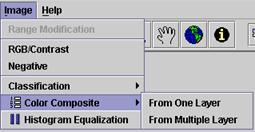
Figure 7. Image Menu

• Help Menu

The “Help” menu allows users to view the user guide and product information.

Figure 8. Help Menu

2.1.2. Tool bar

The tool bar displays buttons that are shortcuts for commonly performed tasks, such as opening and closing a file, zooming in/out of data, and adding or removing data.

Figure 9. Tool Bar

2.1.3. Project tree panel

The tree panel displays the project structure as a tree of "folders". User can click the “tree” node to make data operations, such as displaying data, accessing other value-added Web services.

Figure 10. Project Tree Panel

2.1.4. Data panel

The data panel is where the content of a data object is displayed. All the data are overlaid in the data panel based on geospatial location. More one data object can be displayed in the data panel.

Figure 11. Data Panel

2.1.5. Info panel

The Info panel is used to display data and status information. Data information includes geospatial location. A status message includes file or data downloading information, a warning, or an error message.

Figure 12. Info Panel

2.2. Add Prefer Server List

If accessing data served at certain servers, user should register these server URLs in the preference dialog.

Figure 13. Preference Dialog

1. To open the preference dialog, select menu “Functions -> Preferences”.

2. To add a server URL,enter the URL in the “Server URL” box, and click the “Add” button. The URL will then be on the server list.

3. To delete a server URL, select that server URL in the server list, and click the “Delete” button. The URL will be deleted from the server list.

4. To update a server URL, select a server URL, edit this server URL in the “Server URL” box, and click the “Update” button. The new server URL will be on the server list.

5. After any of the above operations, don’t forget to click the “Apply” button.

6. Click the “OK” button, this dialog will disappear..

7. To add the data in the new server to the data list, select “Services ->UpdateServices ->UpdateCoverage/UpdateFeature/UpdateMap” menu.

2.3. Create a New Project

A project is a group of data files for a specific theme, including coverage data, feature data, and map data, with same the spatial reference system and within the same geospatial bounding box. MPGC allows a user to create a new project or open an existing project and save a project.

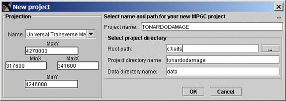
Figure 14. New Project Dialog.

To create a new project, select the menu “File -> New Project” or click to open the “New project” dialog. In this dialog:

Ø Name: the name of spatial reference system.

Ø MinX, MinY, MaxX, MaxY: geospatial bounding box.

Ø Project name: the name of the project.

Ø Root path: project root location.

Ø Project directory name: project directory name. Default, same as project name.

Ø Data directory name: all data are saved in this location. It is under project directory.

Note: the project is saved as a file with the extension of “mpj”.

In our example, the “Projection Name” is “Universal Transverse Mercator” (Note: when you select this name, a new dialog will show for choosing zone. Select zone “18”), the bounding box is “317600, 4246000, 341600 and 4270000”, the “Project name” is “TORNADODAMAGE”, the project path is “c:\laits\tornadodamage\tornadodamage.prj”, and the data file location is “c:\laits\tornadodamage\data”.

3 Coverage Data from Web Coverage Server (WCS)

WCS supports the networked interchange of multi-dimensional and multi-temporal geospatial data as "coverage" through the“getCapabilities”, “describeCoverage” and “getCoverage” interfaces. WCS provides intact geospatial data products encoded in HDF-EOS, NITF and GeoTIFF to meet the requirements of client-side rendering, multi-valued coverages, and input of scientific models, and applicability to clients more complex than simple viewers.

3.1. Getting Coverage Data

To open the coverage browser, select the “Data -> Data Layers” menu or click the toolbar. The “Web Coverage Service Wizard 1” dialog will appear. In this dialog:

Figure 15. Web Coverage Service Wizard 1

Ø Server URLs come either from a CSW service query or from user inputs.

Ø The data layer list for each service is derived from the “getCapabilites” response.

Ø Attributes for each data set, such as bounding box, range set, resolution, and spatial reference system, are derived from the “describeCoverage” response.

When users select data from a data list (in our example, AST_06S_003061820021605_DecorrelationStretchSWIR: band 5, 7, 9 and TM classification are separately selected) and click the “Next” button, the “Web Coverage Service Wizard 2” dialog will show, in which users can subset coverage data in spatial, temporal, resolution/size and range dimensions. In this dialog:

Ø Query parameters

Defines some constraints on query SRS, response SRS, and interpolation method.

Ø Bounding Box/Rectified Coverage

Specifies spatial constraints based on geospatial location or image itself.

Ø Range

Subsets the coverage data by measured quantity or spatial axis. The text in “RangeAxis in Query” always is generated automatically, depending based on the user selection, and it also can be edited for customizing queries.

Ø Resolution/Size

Geospatial resolution or image size of coverage data.

Ø Temporal

Temporal constraints on coverage data.

Depending upon the user’s subsetting of the data attributes, when the “Finish” button is clicked MPGC automatically generates a WCS “getCoverage” request and sends this request to the selected server to get coverage data.

Figure 16. Web Coverage Service Wizard 2

3.2. Operating on Coverage Data

If a coverage is intact data, users can do analysis on the original information included in the coverage. The following operations assume that the user first selects coverage data on the project tree.

3.2.1. Adjusting Palette

If the “Functions -> Palette” menu is selected, the MPGC provides 3 palettes for the coverage data: gray, rainbow, and customized.

Figure 17. Palette Editor

3.2.2. Subsampling

Selecting the menu “Functions -> Subsampling” or clicking the mouse right to select “Subsampling”, users can sub-sample data including adjusting the dimension orientation and dimension size viewing the result in an image or table.

Figure 18. Subsmapling Dialog

3.2.3. RGB Balance Control

If the “Image -> RGB/Contrast” menu is selected, the MPGC will launch an “Image RGB Balance Control” dialog. In this dialog, users can adjust brightness, contrast, RGB balance, the red dimension, the green dimension and the blue dimension of coverage data.

Figure 19. Image RGC Balance Control

3.2.4. Negative

Selecting the “Image -> Negative” menu will display the coverage data in negative form.

3.2.5. Image Classification

MPGC supports unsupervised image classification based on ISODATA. Select one coverage layer, right click mouse to pop up a menu in which select “Web Image Classification Service” or directly select menu “Image -> Classification -> Unsupervised -> ISODATA” (as figure 20), a dialog for image classification will show as figure 21 where “Source URL” is about data location, “Source Format” and “Target Format” mean data format, “numberOfClusters” indicates how many classes will be in the result, and “maxIterationNumber” indicates the maximum iteration number.

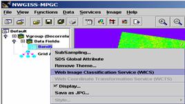
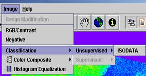
Figure 20. Menus for image classification

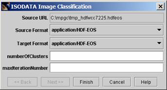
Figure 21. ISODATA image classification dialog

3.2.6. Color Composite

A color composite can be produced for a single coverage data in multiple bands or multi-coverage data with one band.

Note: use “control” key to select multiple coverage data.

If the “Image -> Color Composite -> From One Layer/From Multiple Layer” menu is selected, the “Color Composite” dialog will show. In this dialog, users can specify the correspondence between band/data and dimension and prescribe the scaling method. The result of color composition can be saved as a JPEG file in the project data directory.

Figure 22. Color Composite Dialog

3.2.7. Histogram

4. Feature Data from Web Feature Server (WFS)

Through the “getCapabilities”, “describeFeatureType” and “getFeature” interfaces, WFS supports the networked interchange of geographical vector data as a "feature", which is described by a set of properties, where each property can be thought of as a {name, type, value} tuple, and at least one property is geometry-valued. The name and type of each feature property is determined by its type definition in its schema file. All feature data are encoded in Geographic Markup Language (GML), an extensible markup language for support and storage of geographic vector data to meet the requirements of complex spatial analysis. Currently, the MPGC only supports GML 2.0 in which topology is not included.

4.1. Getting Feature Data

To open the feature browser, select the “Data -> Feature Layers” menu or click the toolbar. The “Web Feature Directory” dialog will appear. In this dialog, users can select different Web feature server and related feature data.

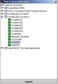
Figure 23. Web Feature Directory Dialog

4.2. Changing Feature Color

If feature data is selected on the project tree, clicking the right mouse and selecting the “Style -> Color” popup menu, will show the “Choose Feature Color” dialog to allow users to change feature color.

Figure 24. Choose Feature Color Dialog

4.3. Getting Feature Information

Every feature in the feature data has its own attribute information, such as ID and name. To get feature information:

Ø Selects a feature data in the project tree panel.

Ø Clicks the toolbar.

Ø Selects a specific feature in the data panel.

Ø Feature information dialog shows.

In our example, there is a damage picture. To show this picture, clicks “SnapShot” attribute in the “feature information” dialog as figure 23.

Figure 25. Feature Information Dialog

5. Map Data from Web Map Server (WMS)

WMS supports the networked interchange of geospatial data as a "map" which is generally rendered dynamically from real geographical data into a spatially referenced pictorial image, such as PNG, GIF or JPEG,. For a digital image map suitable for display on a computer, many organizations, including USGS, NASA, and FGDC are using WMS to publish data. The MPGC provides users an easy way to access thousands of WMSs around the world. The following figure shows the WMS “getMap” user interface in the MPGC, which is launched by selecting the “Data -> Map Layers” menu or clicking the toolbar, where users can specify map data of interest and relevant parameters, such as spatial reference system, bounding box, image size, image format, feature styles for the map, and image transparency.

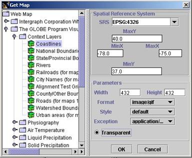
Figure 26. Get Map Dialog

Since image data may be transparent, the map can be overlaid with other data. In the figure 25 the map “coastlines” represented in black line are overlaid above the coverage “Vgroup”.

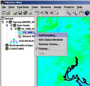
Figure 27. An Example of Map Overlay

6. Service and Data Discovery from Catalog Service for Web (CSW)

Currently CSW as a part of OWS-2 is becoming the de facto standard that supports the registry and discovery of geospatial information resources. It plays a “directory” role in the open, distributed Web service environment: providers register their capabilities using metadata, and users can then query the metadata to discover information of interest. GWSC implements OGC Registry Information model (OGCRIM) and supports the CSW “getRecord” and “getResourceByID” interfaces to allow users to discover distributed services and data by mouse clicking.

To open the catalog browser, click .

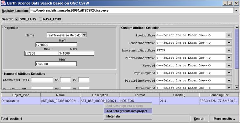
Figure 26. Catalog Browser

In this browser, users can query any known CSW in the MPGC to find interesting data, based on spatial, temporal, topic keyword, platform, instrument and process level attributes rather than data name. Following are the basic operations on CSW to get coverage data.

Discover data

Input constraints on data, such as bounding box, product name and instrument name, click search button to get results.

View data metadata

Select the interested data and right click mouse to select the “Metadata” popup menu.

Add data into project

Select the interested data and right click mouse to select the “Add data granule into project” popup menu, a coverage list dialog will show as figure 27. Usually a data granule can include multiple data coverage. In this dialog, select the interested coverage and right click mouse to select “Add coverage into project” popup menu, a coverage request dialog will show as figure 16 by which data can be downloaded from OGC services and added into project.

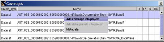
Figure 27 Coverage List Dialog